Rebuilding the Taxi Meter

You do not get to see the rate card. The dataset hands you a fare, a distance, two timestamps, and nothing about how the meter turned the first two into the third. So I fit it backwards. Regress fare on distance and trip duration, read the coefficients, and out falls the meter: a base of $2.74, $2.07 per mile, and 28.4 cents per minute.

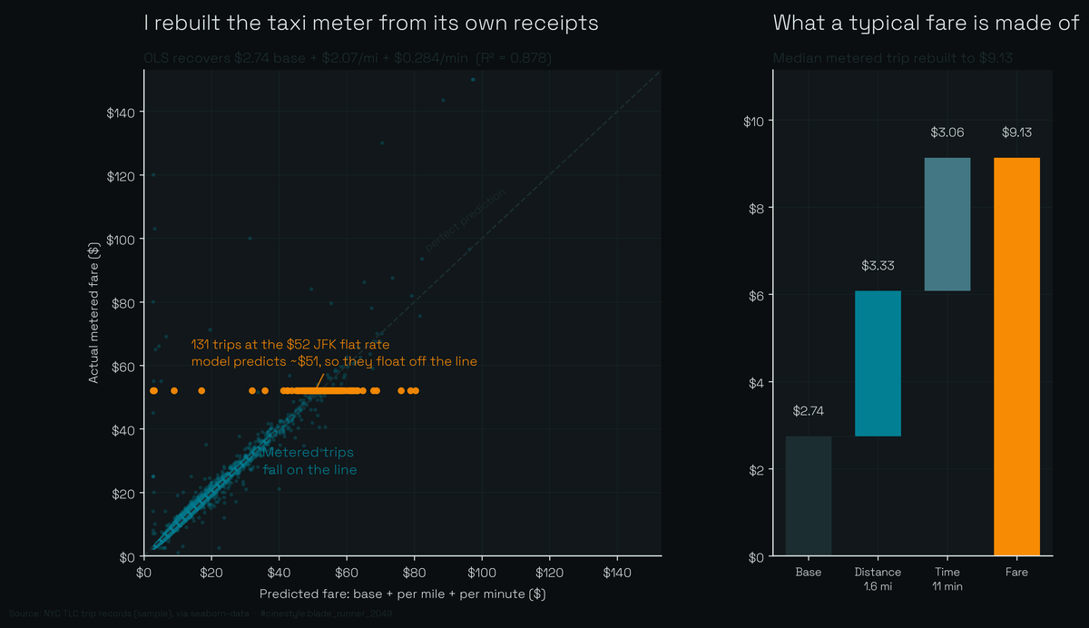
The picture above is the whole argument in one frame. Ordinary least squares recovers the meter to an R² of 0.878, and the metered rides sit on the identity line where a good prediction should put them. The 131 trips charged exactly $52, the old JFK flat rate, refuse to join them. They float off the line as their own band, because a flat fare is not a linear function of anything. That band is the rest of this article.

I am reading coefficients here, not proving causation. The meter is a pricing rule, OLS recovers its dominant linear shape, and that is all I am claiming. The interesting part is the one time in five it misses, because the misses are not noise. They are a second pricing system the meter is hiding inside a single column.

The setup

This is the seaborn-data sample of NYC TLC trip records, 6,433 yellow- and green-cab rides from a window in early 2019, with pickup and dropoff timestamps, distance, fare, tip, tolls, total, zones, and payment type. I derived trip duration as dropoff minus pickup. Six rows came back with zero or negative duration, clock skew, or a meter that closed before it opened, so I dropped them and modeled the remaining 6,427. No fares were missing or non-positive.

The honest caveat shapes everything below. This is 6k rows from one month, and my model has no surge multiplier, no rush-hour term, no night surcharge, no tolls in the fit. NYC’s real meter has all of those. So when I say I recovered the rate, I mean I recovered the dominant linear part of it. The structure I am about to point at is the part that survives that simplification, which is exactly why I trust it.

The regression that worked

Fitting fare ~ distance + duration_min by ordinary least squares gives an R² of 0.878. The two terms split the work cleanly: $2.07 per mile (95% CI $2.03 to $2.12) and $0.284 per minute (CI $0.269 to $0.298), over a base of $2.74.

Both terms earn their place. Distance alone already explains 85.1% of the variance, so duration is only buying me another three points of R², but it is buying real ones. A taxi that is moving charges you for ground covered. A taxi stuck in traffic charges you for time. The per-minute term is the meter ticking while you sit at a light. There is a speed where the two cost you the same: at $0.284 per minute and $2.07 per mile, the time charge equals the distance charge at about 8 miles an hour. Below that you pay mostly for time, above it mostly for distance. Manhattan traffic lives right around there, which is why both terms matter.

The residuals are clean. Mean residual is zero by construction, but the median absolute residual is just $0.48, and the residuals carry essentially no leftover correlation with distance or duration (both round to 0.00). The linear model has wrung out the linear signal. What is left is either random or not linear, and the not-linear part is where this gets interesting.

The 85% that fits, and the 15% that does not

Put a band of plus-or-minus one dollar around the prediction. 5,472 of 6,427 trips, 85.1%, land inside it. Widen to $2 and you capture 94.6%. The typical ride is a solved problem: the reconstructed meter predicts it to within pocket change.

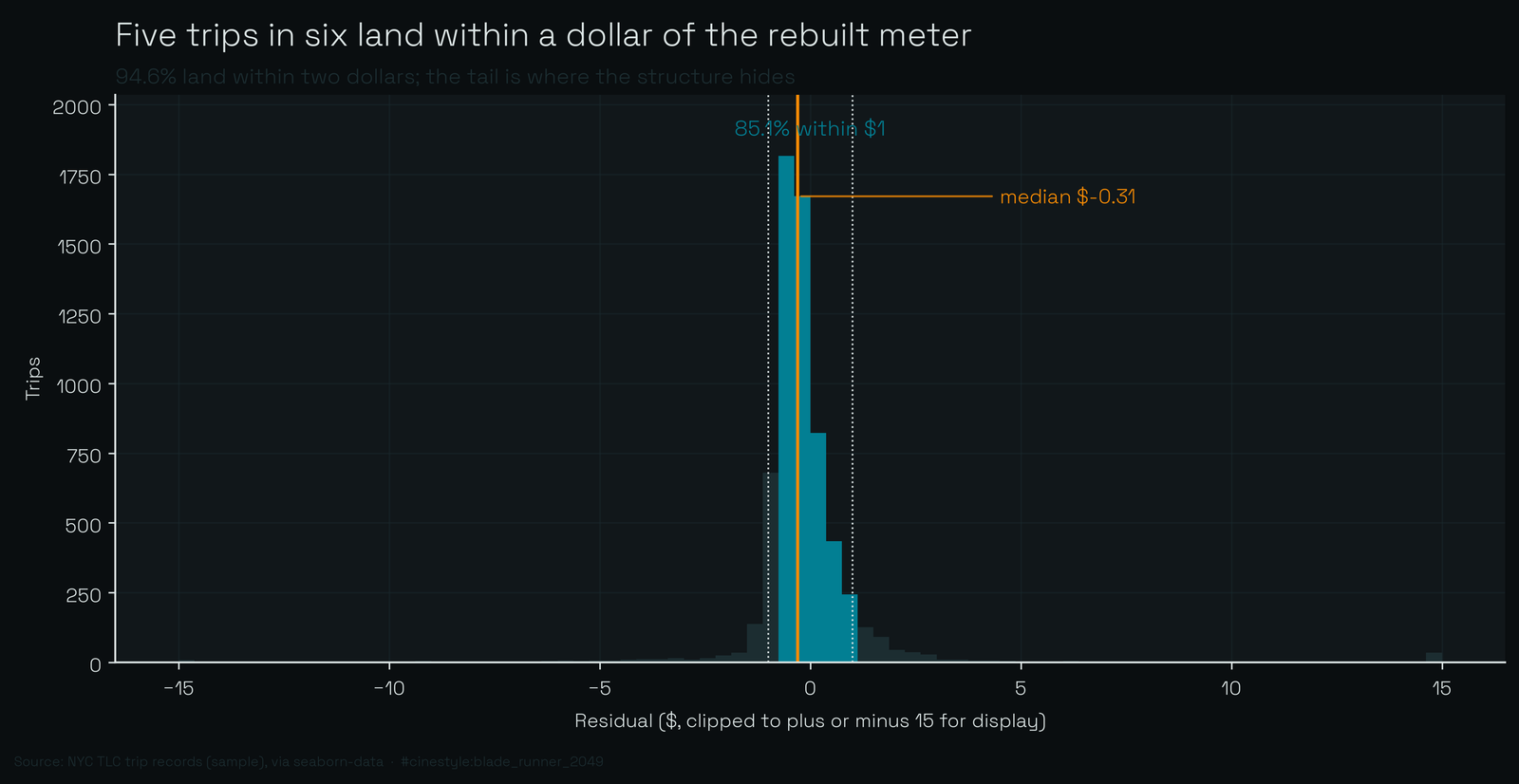
But 955 trips fall outside the dollar band, and they do not scatter randomly. Plot the residual against distance and a horizontal streak jumps out, far up the distance axis, floating well above the zero line.

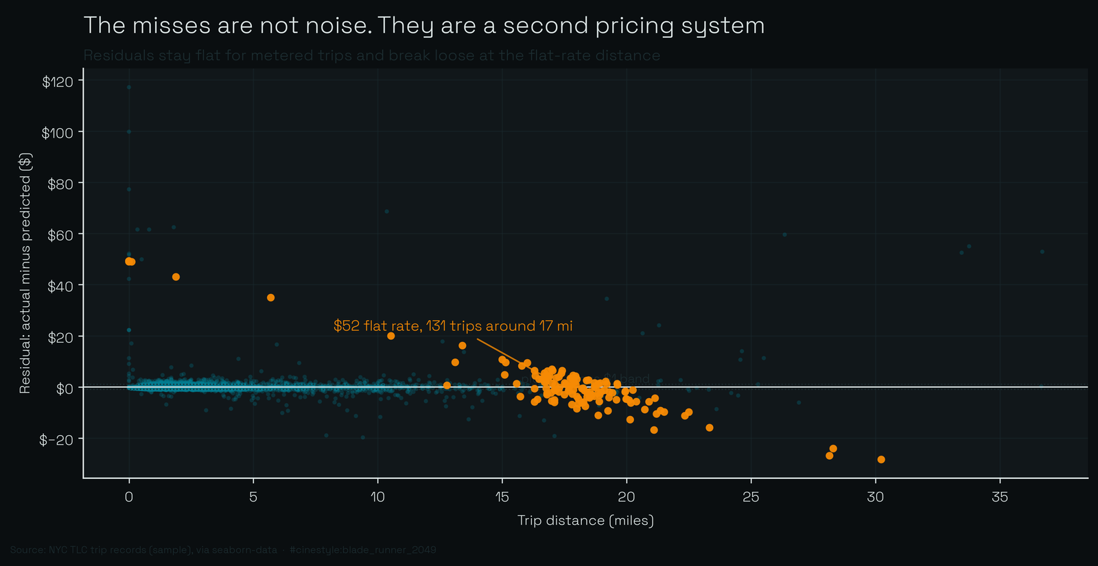
Those are the airport trips. 131 rides in the sample charged exactly $52.00, the old JFK-to-Manhattan flat fare. They average 17.2 miles, and a flat fare is by definition not a linear function of distance, so my linear model has no hope of nailing them. It predicts $50.65 on average and misses by a dollar and change either way depending on how far the particular trip ran. Of the 955 trips outside the dollar band, 119 are these $52 flats, 12.5% of all my misses concentrated in one fixed price point. The flat-rate regime is a second meter bolted onto the first, and it accounts for an eighth of everywhere my reconstruction breaks.

Where it breaks worst

Two smaller pathologies sit at the extremes. 45 trips logged zero distance but a positive fare: meter started, GPS never moved, or the ride got cancelled after the flag drop. Their median fare is $3.50, right at a base-plus-a-minute charge, but their mean is $20.93, because a few of them billed long durations with no distance. The model, leaning hard on a distance it is told is zero, under-predicts them by an average of $17.35. Those are the single worst residuals in the set. The largest is a trip the meter charged $117 more than my model expected.

The other edge is the short hops. I pulled the 119 rides under two minutes and under half a mile, the ones where the base fare should dominate everything. The median fare there is $3.00 and the model predicts $3.38, basically perfect, the base fare doing its job. But the mean residual for that group is +$6.84, and that surprised me until I looked: six of those 119 short trips are $52 flat-rate fares with a mis-logged near-zero distance, and the group’s max fare is $120. A handful of records poison the average of an otherwise tidy group. The median tells the true story and the mean tells you the data is dirty. Both are worth knowing.

What the residuals are really telling you

The real lesson is that fare is two columns wearing one hat. There is a metered regime, linear in distance and time, recoverable to the cent, 85% of the rides. There is a flat-rate regime stamped on top of it that the linear fit can only ever smear across. If you are building anything on this data, a duration model, an anomaly detector, a fraud check, you want a flat-rate flag carried explicitly, because the meter will not hand you one and the residuals are the only place it leaks.

I went in expecting to recover a rate. I did: $2.07 a mile, 28 cents a minute. What I did not expect was that the cleanest way to find the airport pricing was not to look for it. It was to fit the wrong model on purpose and read what it could not explain.