The Cancer Decision Threshold

Accuracy is the wrong scoreboard for a cancer screen, and 0.5 is the wrong place to stand. At a 0.5 cutoff my logistic regression missed 4 of the 64 malignant tumors in the test set. Four women told they are fine when they are not. The model’s accuracy was 97.1%, its AUC 0.9975, and on any benchmark leaderboard those numbers close the case. But 0.5 is a default inherited from predict, not a clinical decision, and it quietly optimizes for the error you care least about.

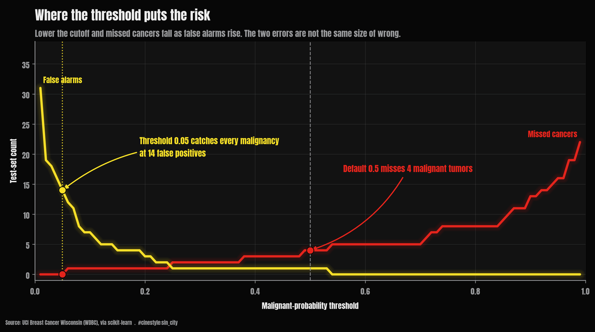
The whole argument is in that one chart. The red line is missed cancers, the yellow line is false alarms, and they move in opposite directions as you slide the cutoff. At 0.5 the red line sits at four. Drop the cutoff to 0.05 and it hits zero, while the yellow line climbs to fourteen. The question is never which line to minimize. It is which mistake you can afford to make.

The data is the Breast Cancer Wisconsin (WDBC) set bundled with scikit-learn: 569 fine-needle-aspirate samples, 30 nucleus-shape features, sourced from UCI. Of those, 212 are malignant and 357 benign. One thing to nail down before anything else. In this version target=0 is malignant and target=1 is benign, the opposite of the intuitive coding. I did not trust the docs, so I checked. Mean nucleus radius is 17.46 for class 0 and 12.15 for class 1. Malignant tumors have bigger nuclei, so class 0 is malignant. I recoded so malignant is the positive class (1), because the thing you are trying to catch should be the thing the model calls positive.

The setup, and the metric trap

I split 70/30, stratified, fixed seed, and put the StandardScaler inside the pipeline so it only ever fits on training rows. No leakage. The held-out test set is 171 samples: 64 malignant, 107 benign. Logistic regression, nothing fancy.

At the default 0.5 threshold the confusion matrix is: 106 true negatives, 60 true positives, 1 false positive, and 4 false negatives. Read that last number again. Sensitivity for malignant, the fraction of cancers the model actually flags, is 93.75%. The model is excellent at saying “this is benign and I’m right” and it is stingy with false alarms, one in total. It pays for that stinginess in the only currency that matters here. It lets four cancers walk.

This is the trap. Accuracy and AUC both reward the model for being confidently correct on the easy benign majority. Neither asks what the one kind of mistake you cannot afford costs you. A false positive here means a scared patient and a follow-up biopsy. A false negative means a missed malignancy. Those are not the same magnitude of wrong, and treating the confusion matrix as symmetric, which is what 0.5 does, bakes in the assumption that they are. A symmetric metric on an asymmetric problem will always sell you the cheap error.

Move the line

The fix is not a better model. It is a different operating point. The predicted probability is a continuous score, and 0.5 is just one place to cut it. Lower the malignant-probability threshold and you convert false negatives into true positives, at the price of more false positives.

The probability histogram shows why this works and where it stops working. Picture the test set sliding down a funnel onto the probability axis: most benign cases pool near 0, most malignant near 1, and the dangerous cases are the malignant ones that drift into the benign pool. They do not cleanly separate. There is a smear of malignant cases sitting below 0.5, and those are exactly the four the default cutoff misses. They are not all hugging the line either. The lowest-scoring malignant case in the test set lands at a predicted probability of 0.0591, down in the benign pile, which is the uncomfortable part. Catching it means sweeping in every benign case that scores that low too.

Here is the sweep, in the numbers I would actually show a stakeholder:

threshold	false negatives	false positives	sensitivity	specificity
0.50	4	1	0.938	0.991
0.30	2	1	0.969	0.991
0.20	1	3	0.984	0.972
0.10	1	7	0.984	0.935
0.05	0	14	1.000	0.869

Drop from 0.5 to 0.20 and the missed cancers fall from four to one. The cost is two extra false positives, 3 instead of 1. That is the cheapest, most defensible move on the whole curve. You cut misses by 75% for two more benign biopsies. Keep going to 0.05 and you catch every single malignant tumor in the test set. Zero false negatives. The bill for that perfection is 14 benign cases flagged, up from 1. Thirteen extra women sent for a follow-up they did not need, to make sure nobody with cancer gets sent home. On this problem, the follow-up is the affordable mistake.

What 100% recall actually costs

I asked the script for the highest threshold that still catches every malignancy, because a higher threshold means fewer false alarms for the same recall. It is 0.05. At that point specificity drops to 0.869, so about 13% of benign patients get flagged. Whether that trade is worth it is not a modeling question. It is a question for whoever owns the consequences. But the model cannot even pose it at 0.5, because at 0.5 the four misses are invisible inside a 97% accuracy figure that looks like a win.

One honest wrinkle. In my test set there is no threshold that buys you a tidy 99%-recall operating point distinct from 100%. The sweep jumps from one missed cancer (sensitivity 0.984) straight to zero. That is not a deep property of the model. It is that 64 malignant test cases means each one is worth 1.6 percentage points of sensitivity, so the curve moves in chunky steps. With a bigger test set the staircase would smooth out. It is a reminder that these clean second-decimal-place numbers are estimated on 171 rows, and the confidence interval around “97.1% accuracy” is wider than the precision implies.

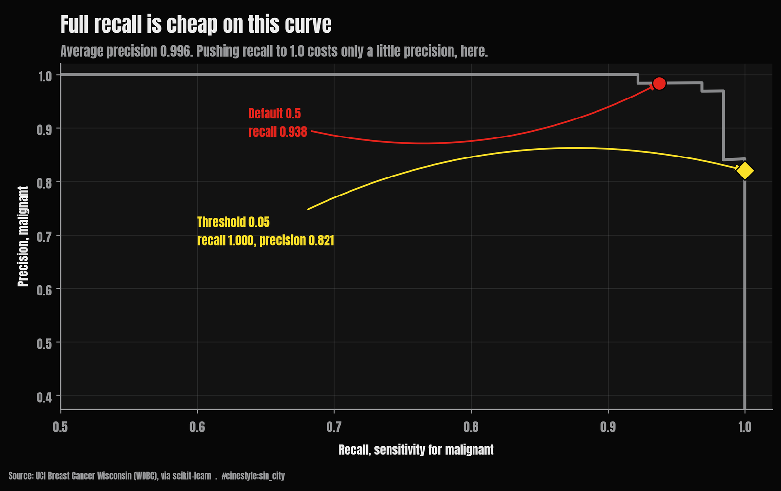
The average precision is 0.9963 and the AUC 0.9975, so this is a near-ceiling classifier on a famously clean benchmark. The features were hand-engineered from segmented microscope images by people who already knew what malignancy looks like. The classes are only mildly imbalanced. There is no missingness, no label noise, no drift between sites. Real screening pipelines have all of that, and this is not a medical device. It is a logistic regression on a teaching dataset. What survives the move to the real world is not the specific threshold. It is the discipline. Pick the operating point from the cost of the two errors, then read accuracy afterward as a footnote. The default 0.5 already made that decision for you, and it decided four missed cancers was an acceptable price for one fewer false alarm.